Uncrossing lines
This is the sixth post in an open-ended series on proving the correctness of TLA specifications using Isabelle/HOL:
-
Uncrossing lines
Introduction
I recently came across a video lecture by Dijkstra on reasoning about program correctness in which he discusses two little algorithms that have interesting correctness proofs. The first has a slightly surprising safety (i.e. partial correctness) property, but is very easy to show that it terminates, whereas the second has an obvious safety property but a trickier termination proof. I thought it’d be interesting to code the second up in TLA and play around with it.
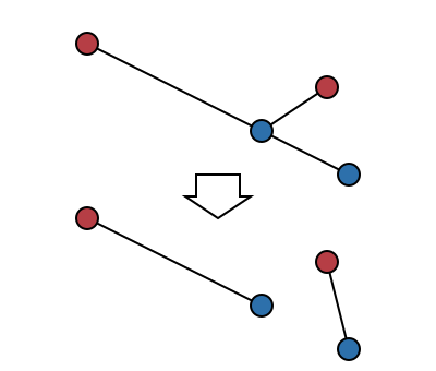
The setup is that there are n red points and n blue points in the plane, where each red point is joined to a blue point by a straight line segment:
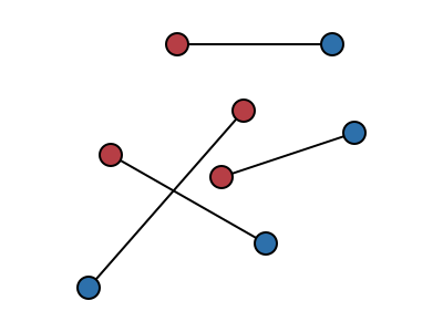
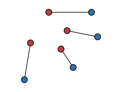
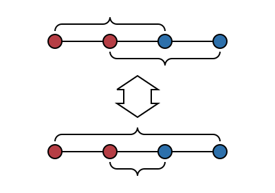
The objective is to find a way of pairing up the red points with the blue points so that none of the line segments cross. The algorithm to do this starts with any pairing and repeatedly selects a pair of line segments which cross and “uncrosses” them, swapping the pairings between the two red points and the corresponding blue points:
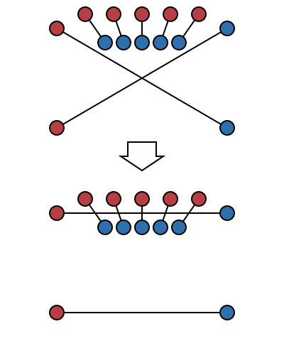
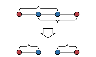
Since the algorithm repeats until there are no crossing line segments, if it terminates then it has successfully found an arrangement with no crossing segments. In other words, it’s easy to see that this algorithm has a good partial correctness property. However it’s not immediately obvious that this algorithm does ever terminate. It’s tempting to want to try something like induction on the number of crossing pairs of segments: the act of uncrossing a pair of segments certainly removes one crossing, but the problem with this approach is that an uncrossing can also introduce arbitrarily many other crossings, so this induction doesn’t work:
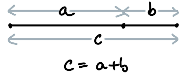
As there are only finitely many points there are only finitely many arrangements from which to choose, so if the algorithm fails to terminate then it must repeatedly visit the same state. The trick is to notice that uncrossing two crossing lines always makes the total length of all the lines strictly shorter, so it’s not possible to visit any state more than once. This is because of the triangle inequality:
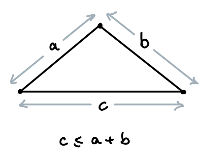
Actually it isn’t always true that the total length always gets shorter: the triangle inequality is only strict if the triangle is not degenerate, i.e. if its vertices are not collinear.
And indeed it’s possible to find cases where the four points involved in an uncrossing are all collinear, the lines intersect, and yet swapping the pairings over does not decrease the total length of the lines or remove the intersection:
Does this count as “crossing”? Arguably no, two line segments are “crossing” only if there is some of each line segment lies on both sides of the other, which isn’t the case if the endpoints are collinear. But they do intersect, which is a little more general, and there are some other cases where the line segments intersect (but don’t strictly cross) and where swapping the pairing of the endpoints does remove the intersection:
Dijkstra avoids this whole issue by insisting that of all the red and blue points no three of them are collinear, which excludes the problematic case but also the case above; also if only three of the four endpoints involved in an intersection are collinear then swapping the pairing always decreases the total length and removes the intersection:
It turns out that we can be a bit more precise about the conditions under which this algorithm works.
This post is a tour of
EWD-pairings.thy
in my TLA examples Github
repository.
Geometry in Isabelle/HOL
There seems to be a surprisingly small amount of geometry included in the Isabelle/HOL standard library. There’s a theory of real numbers, and of vector spaces which specialises to ℝ², including the (non-strict) triangle inequality, but I couldn’t find much about lines and their intersections and so on, so I started with these definitions:
type_synonym point = "real × real"

definition lineseg :: "point ⇒ point ⇒ real ⇒ point"
  where "lineseg p0 p1 l ≡ (1-l) *R p0 + l *R p1"
  (* The *R operator is scalar multiplication *)

definition closed_01 :: "real set"
  where "closed_01 ≡ {x. 0 ≤ x ∧ x ≤ 1}"

definition segment_between :: "point ⇒ point ⇒ point set"
  where "segment_between p0 p1 ≡ lineseg p0 p1 ` closed_01"

definition segments_cross :: "point ⇒ point ⇒ point ⇒ point ⇒ bool"
  where "segments_cross r0 b0 r1 b1
       ≡ segment_between r0 b0 ∩ segment_between r1 b1 ≠ {}"
In words, lineseg p0 p1 is a function real ⇒ point whose range is the line
through p0 and p1, and segment_between p0 p1 is the segment of this line
between p0 and p1 (inclusive). The property we care about is whether the
two segments intersect, given by segments_cross.
Starting from these definitions I did manage to show that, if no three points are collinear, then uncrossing two crossing segments does indeed decrease the sums of their lengths, but it was quite a long and unilluminating proof so I started casting around for examples of other geometry that has been developed in Isabelle/HOL to see if there were any better ideas.
Signed areas
I came across Laura I. Meikle’s PhD thesis which uses formalisation of geometric results as a running example to motivate various usability improvements in automated proof tooling. Included is a substantial formalisation of a convex hull algorithm, including novel work to show that the algorithm works if some points are collinear, which seems to be considered as something of a special case in computational geometry even though I imagine it occurs quite often in practice. This motivated me to try a little harder and dig into the cases where some of the points could be collinear and try and isolate just the problematic cases of collinearity.
The basic idea of Meikle’s formalisation, apparently from Knuth’s Axioms and Hulls, is to use the idea of signed area to classify arrangements of three points. The signed area is the area of the triangle whose vertices are the three points, if ordered anticlockwise, or the negation of its area if the points are clockwise. This has a particularly simple formula in terms of the coordinates of the points:
definition signedArea :: "point ⇒ point ⇒ point ⇒ real"
  where "signedArea p0 p1 p2 ≡ case (p0, p1, p2) of
    ((x0,y0), (x1,y1), (x2,y2)) ⇒ (x1-x0)*(y2-y0) - (x2-x0)*(y1-y0)"
(In fact this gives twice the area of the triangle in question, but really we
mostly only care about the sign, and the extra factor of ½ makes everything
harder, so it’s better just to leave it out). The key point is that if
signedArea p0 p1 p2 is negative then p2 is to the left of the directed line
segment from p0 to p1 and if it is positive then p2 is to the right:
lemma signedArea_left_example:  "signedArea (0,0) (1,0) (1, 1) > 0" by (simp add: signedArea_def)
lemma signedArea_right_example: "signedArea (0,0) (1,0) (1,-1) < 0" by (simp add: signedArea_def)
If the signed area is zero then the points are collinear. Since we mostly only care about the sign of the signed area, it makes sense to throw away its magnitude like this:
datatype Turn = Left | Right | Collinear

definition turn :: "point ⇒ point ⇒ point ⇒ Turn"
  where "turn p0 p1 p2 ≡ if 0 < signedArea p0 p1 p2 then Left
                          else if signedArea p0 p1 p2 < 0 then Right
                          else Collinear"
One cute fact about signed areas is that they interact nicely with the linear
interpolation used in lineseg. Recalling that lineseg r1 b1 l ≡ (1-l) *R r1 + l *R b1,
it follows that:
lemma signedArea_lineseg:
    "signedArea r0 b0 (lineseg r1 b1 l)
        = (1-l) * signedArea r0 b0 r1
           + l  * signedArea r0 b0 b1"
Classifying crossing segments
A bunch of preliminary results lead to a quite neat classification of crossing segments in terms of their turn directions:
lemma segments_cross_turns:
  assumes "segments_cross r0 b0 r1 b1"
  shows "collinear {r0, b0, r1, b1}
       ∨ (turn r0 b0 r1 ≠ turn r0 b0 b1
        ∧ turn r1 b1 r0 ≠ turn r1 b1 b0)"
This means that two line segments intersect either when all four points are collinear, or else when the two endpoints of each line segment are on different sides of the other line, and what’s really nice is that this includes cases where some of the points are collinear: “different sides” means “left and right” or “left and collinear” or “right and collinear”. In this latter case the segments do genuinely cross …
lemma turns_segments_cross:
  assumes "turn r0 b0 r1 ≠ turn r0 b0 b1"
  assumes "turn r1 b1 r0 ≠ turn r1 b1 b0"
  shows "segments_cross r0 b0 r1 b1"
… and swapping the endpoints does decrease the length:
lemma non_collinear_swap_decreases_length:
  assumes distinct:       "r0 ≠ r1" "b0 ≠ b1"
  assumes distinct_turns: "turn r0 b0 r1 ≠ turn r0 b0 b1"
                          "turn r1 b1 r0 ≠ turn r1 b1 b0"
  shows "dist r0 b1 + dist r1 b0 < dist r0 b0 + dist r1 b1"
The side-conditions r0 ≠ r1 and b0 ≠ b1 are necessary: without them,
swapping endpoints doesn’t change the line segments. In the algorithm we do not
allow line segments to share endpoints.
Dealing with collinear points
The cases where the segments intersect and all four points are collinear are easy enough to enumerate:
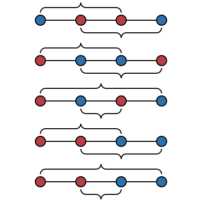
Of these, the only cases in which swapping the endpoints does not decrease the total length, or remove the intersection, is the last two in which both of the blue points are on the same side of the two red points. This suggests the following definition to try and exclude the problematic case:
definition badly_collinear :: "point ⇒ point ⇒ point ⇒ point ⇒ bool"
  where "badly_collinear r0 b0 r1 b1
          ≡ ({b0,b1} ⊆ lineseg r0 r1 ` { l. 1 < l }
           ∨ {b0,b1} ⊆ lineseg r1 r0 ` { l. 1 < l })"
It’s not too hard to show that this is a very problematic case, in the sense that it means that the line segments intersect …
lemma badly_collinear_intersects:
  assumes "badly_collinear r0 b0 r1 b1"
  shows "segments_cross r0 b0 r1 b1"
… you can’t escape by swapping the endpoints …
lemma badly_collinear_swap_still_badly_collinear:
  assumes "badly_collinear r0 b0 r1 b1"
  shows   "badly_collinear r0 b1 r1 b0"
… and swapping the endpoints doesn’t change the total length of the segments …
lemma badly_collinear_swap_preserves_length:
  assumes bad: "badly_collinear r0 b0 r1 b1"
  shows "dist r0 b1 + dist r1 b0 = dist r0 b0 + dist r1 b1"
… which means that this case definitely prevents the algorithm from terminating. However, it’s also possible to show that this is the only situation that can prevent the algorithm from terminating:
lemma swap_decreases_length:
  assumes distinct:       "distinct [r0, b0, r1, b1]"
  assumes segments_cross: "segments_cross r0 b0 r1 b1"
  assumes not_bad:        "¬ badly_collinear r0 b0 r1 b1"
  shows "dist r0 b1 + dist r1 b0 < dist r0 b0 + dist r1 b1"
The proof of this is a slightly fiddly set of nested case splits of the form that Isabelle excels at compared with doing this manually. It’s really hard to convince yourself you’ve got all the cases, particularly when working geometrically, as some of the case splits yield geometrically-impossible situations which can’t be drawn but which you still have to prove to be impossible.
Setting up the algorithm
The analysis above suggests the following setup for modelling the algorithm itself:
locale UncrossingSetup =
  fixes redPoints bluePoints :: "point set"
  assumes finite_redPoints:  "finite redPoints"
  assumes finite_bluePoints: "finite bluePoints"
  assumes cards_eq:  "card redPoints = card bluePoints"
  assumes red_blue_disjoint: "redPoints ∩ bluePoints = {}"
  assumes not_badly_collinear:
      "⋀r1 r2. ⟦ r1 ∈ redPoints; r2 ∈ redPoints ⟧
          ⟹ card (bluePoints ∩ lineseg r1 r2 ` {l. 1 < l}) ≤ 1"
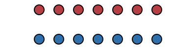
The condition not_badly_collinear says that if you draw a line segment
between any two red points, and extend it past one of the red points, then it
only ever hits at most one blue point. This allows for a lot more situations
than simply forbidding any collinearity. For instance, all the red points can
be collinear, as can all the blue points:
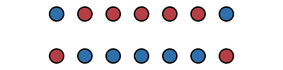
It’s also permissible to have a bunch of blue points on the line between two red points and vice versa:
In this setup, any uncrossing reduces the total length of the line segments involved:
context UncrossingSetup
begin

lemma uncross_reduces_length:
  fixes r1 r2 b1 b2
  assumes colours: "r1 ∈ redPoints" "r2 ∈ redPoints" "b1 ∈ bluePoints" "b2 ∈ bluePoints"
  assumes distinct: "r1 ≠ r2" "b1 ≠ b2"
  assumes segments_cross: "segments_cross r1 b1 r2 b2"
  shows "dist r1 b2 + dist r2 b1 < dist r1 b1 + dist r2 b2"
Moreover the total length of any pairing of the red points and the blue points is in this set…
definition valid_total_lengths :: "real set"
  where "valid_total_lengths
    ≡ (λpairs. ∑ pair ∈ pairs. dist (fst pair) (snd pair))
          ` Pow (redPoints × bluePoints)"
… which is finite …
lemma finite_valid_total_lengths: "finite valid_total_lengths"
… so this means that transitions which reduce the total length form a wellfounded relation, suitable for induction:
definition valid_length_transitions :: "(real × real) set"
  where "valid_length_transitions ≡ Restr {(x,y). x < y} valid_total_lengths"

lemma wf_less_valid_total_length: "wf valid_length_transitions"
The algorithm
At this point we are in a position to look at the algorithm itself in TLA:
definition swapPoints :: "point ⇒ point ⇒ point ⇒ point"
  where "swapPoints p0 p1 p ≡ if p = p0 then p1 else if p = p1 then p0 else p"

locale Uncrossing = UncrossingSetup +
  fixes blueFromRed :: "(point ⇒ point) stfun"
  assumes bv: "basevars blueFromRed"
  fixes blueFromRed_range :: stpred
  defines "blueFromRed_range
      ≡ PRED ((op `)<blueFromRed,#redPoints> = #bluePoints)"
  fixes step :: action
  defines "step ≡ ACT (∃ r0 r1 b0 b1.
              #r0 ∈ #redPoints
            ∧ #r1 ∈ #redPoints
            ∧ #r0 ≠ #r1
            ∧ #b0 = id<$blueFromRed,#r0>
            ∧ #b1 = id<$blueFromRed,#r1>
            ∧ #(segments_cross r0 b0 r1 b1)
            ∧ blueFromRed$ = (op ∘)<$blueFromRed,#(swapPoints r0 r1)>)"
  fixes Spec :: temporal
  defines "Spec ≡ TEMP (Init blueFromRed_range ∧ □[step]_blueFromRed
                          ∧ WF(step)_blueFromRed)"
We have a single state variable, blueFromRed, which assigns the corresponding
blue point to each red point. The predicate blueFromRed_range holds
initially, and each (non-stuttering) transition finds two intersecting line
segments and uncrosses them. The expression
blueFromRed$ = (op ∘)<$blueFromRed,#(swapPoints r0 r1)>)"
is the Isabelle translation of what would be written in TLA+ something like
blueFromRed' = blueFromRed ∘ (swapPoints r0 r1)
i.e. that updating the blueFromRed function simply swaps an assignment over
and leaves everything else alone, and the predicate blueFromRed_range is a
translation of
blueFromRed ` redPoints = bluePoints
i.e. that blueFromRed is a surjection from the red points onto the blue points (and these sets are finite and have equal cardinalities which means it’s a bijection). It’s not too hard to show that this predicate is an invariant of the algorithm:
lemma blueFromRed_range_Invariant: "⊢ Spec ⟶ □blueFromRed_range"
Furthermore it implies that the total length of all the line segments is in
valid_total_lengths:
definition total_length :: "real stfun"
  where "total_length s ≡ ∑ r ∈ redPoints. dist r (blueFromRed s r)"

lemma blueFromRed_range_valid_total_length:
  "⊢ blueFromRed_range ⟶ total_length ∈ #valid_total_lengths"
We can define what it means for all the line segments to be uncrossed:
definition all_uncrossed :: stpred
  where "all_uncrossed ≡ PRED (∀ r0 r1 b0 b1.
              #r0 ∈ #redPoints
            ∧ #r1 ∈ #redPoints
            ∧ #r0 ≠ #r1
            ∧ #b0 = id<blueFromRed,#r0>
            ∧ #b1 = id<blueFromRed,#r1>
            ⟶ ¬ #(segments_cross r0 b0 r1 b1))"
It follows that the algorithm can only stutter once all line segments are uncrossed:
lemma stops_when_all_uncrossed:
  "⊢ Spec ⟶ □($all_uncrossed ⟶ blueFromRed$ = $blueFromRed)"
All of the preliminary work above allows us to show that a step transition
causes the change in total_length to be in valid_length_transitions:
lemma step_valid_length_transition:
  assumes "(s,t) ⊨ step"
  assumes "s ⊨ blueFromRed_range"
  shows "(total_length t, total_length s) ∈ valid_length_transitions"
From this, and because valid_length_transitions is a wellfounded relation,
there can only be finitely many step transitions, which means that eventually
the algorithm does terminate as required.
lemma "⊢ Spec ⟶ ◇□all_uncrossed"
Conclusion
This algorithm is interesting because its correctness proof relies on a geometric argument, something that I’d not seen before. The actual computational content (i.e. the interaction with TLA) was quite small and simple, once the geometry was all sorted out.
I’ve never done any formalisation of geometry before, and the idea of signed
areas helped to show me a way of working that was a lot more elegant than the
bare-hands coordinate geometry that I initially tried. It also helped
massively in the analysis of the problematic situations involving collinear
points. For these situations it was very useful to work in Isabelle as there
were a few places where I had to proceed by enumerating cases and it’s all to
easy to miss one case when working by hand, especially when working with
geometry and doubly so when trying to consider degenerate cases. The proof of
swap_decreases_length in particular involved nested case splits that would
have been tricky to cover exhaustively by hand.
This algorithm works in terms of real numbers, which made it simple to analyse
but means it cannot be implemented as-is. Naively replacing all the real
numbers with floating-point double variables seems like it’ll give rise to
some problems, particularly for points that are close to collinear, in part
because the formula for signedArea has lots of subtractions of quantities
that could be quite similar. This needs more thought as I haven’t yet been able
to construct an obviously-bad situation for double variables, so bad
behaviour is just a hunch. An obvious cop-out is to compute exactly using
integer or rational coordinates instead.